Jacob Freedman's Portfolio
webpage portfolio for open source GIS work
Project maintained by jafreedman12 Hosted on GitHub Pages — Theme by mattgraham
RP- Vulnerability modeling for sub-Saharan Africa
Reproduction of
Vulnerability modeling for sub-Saharan Africa
Original study by Malcomb, D. W., E. A. Weaver, and A. R. Krakowka. 2014. Vulnerability modeling for sub-Saharan Africa: An operationalized approach in Malawi. Applied Geography 48:17–30. DOI:10.1016/j.apgeog.2014.01.004
Reproduction Authors: Jacob Freedman, Joseph Holler, Kufre Udoh, Open Source GIScience students of fall 2019 and Spring 2021 Co-created with Alitzel Villanueva, Arielle Landau, Drew An-Pham, Emma Clinton, Maja Cannavo, and Nick Nonnenmacher
Reproduction Materials Available at: RP-Malcomb
Created: 12 April 2021
Revised: 27 April 2021
Abstract
The original study is a multi-criteria analysis of vulnerability to Climate Change in Malawi, and is one of the earliest sub-national geographic models of climate change vulnerability for an African country. The study aims to be replicable, and had 40 citations in Google Scholar as of April 8, 2021.
Original Study Information
The study region is the country of Malawi. The spatial support of input data includes DHS survey points, Traditional Authority boundaries, and raster grids of flood risk (0.833 degree resolution) and drought exposure (0.416 degree resolution).
The original study was published without data or code, but has detailed narrative description of the methodology. The methods used are feasible for undergraduate students to implement following completion of one introductory GIS course. The study states that its data is available for replication in 23 African countries.
Data Description and Variables
This component was written collaboratively with Alitzel Villanueva, Maja Cannavo, Emma Clinton, Drew An-Pham, and Nick Nonnenmacher, all students in GEOG0323.
Assets and Access:
Demographic and Health Survey data are a product of the United States Agency for International Development (USAID). Variables contained in this dataset are used to represent adaptive capacity (access + assets) in the Malcomb et al.’s (2014) study. These data come from survey questionnaires with large sample sizes.
The DHS data used in our study were collected in 2010. In Malawi, the provenance of the DHA data dates back as far as 1992, but has not been collected consistently every year. Each point in the household dataset represents a cluster of households with each cluster corresponding to some form of census enumeration units, such as villages in rural areas or city blocks in urban areas DHS GPS Manual. This means that each household in each cluster has the same GPS data. This data is collected by trained USAID staff using GPS receivers.
Missing data is a common occurrence in this dataset as a result of negligence or incorrect naming. However, according to the DHS GPS Manual, these issues are easily rectified and typically sites for which data does not exist are recollected. Sometimes, however, missing information is coded in as such or assigned a proxy location.
The DHS website acknowledges the high potential for inconsistent or incomplete data in such broad and expansive survey sets. Missing survey data (responses) are never estimated or made up; they are instead coded as a special response indicating the absence of data. As well, there are clear policies in place to ensure the data’s accuracy. More information about data validity can be found on the DHS’s Data Quality and Use site.
In this analysis, we use the variables listed in Table 1 to determine the average adaptive capacity of each TA area. Data transformations are outlined below.
Table 1: Variables from DHS data
| Variable Code | Definition |
|---|---|
| HHID | “Case Identification” |
| HV001 | “Cluster number” |
| HV002 | Household number |
| HV246A | “Cattle own” |
| HV246D | “Goats own” |
| HV246E | “Sheep own” |
| HV246G | “Pigs own” |
| HV248 | “Number of sick people 18-59” |
| HV245 | “Hectares for agricultural land” |
| HV271 | “Wealth index factor score (5 decimals)” |
| HV251 | “Number of orphans and vulnerable children” |
| HV207 | “Has Radio” |
| HV243A | “Has a Mobile Telephone” |
| HV219 | Sex of Head of Household” |
| HV226 | “Type of Cooking Fuel” |
| HV206 | “Has electricty” |
| HV204 | “Time to get to Water Source” |
Livelihood Zones:
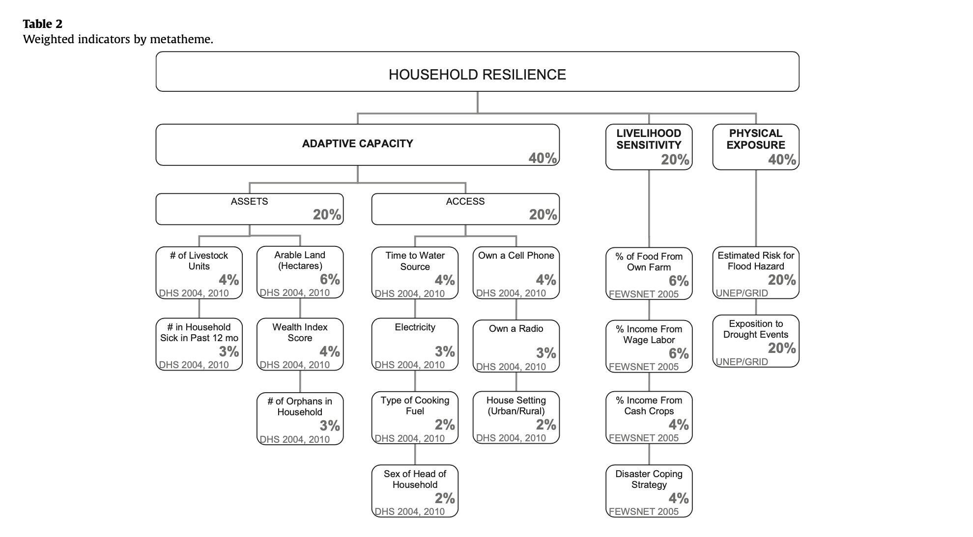
The Livelihood zone data is created by aggregating general regions where similar crops are grown and similar ecological patterns exist. This data exists originally at the household level and was aggregated into Livelihood Zones. To construct the aggregation used for “Livelihood Sensitivity” in this analysis, we use these household points from the FEWSnet data that had previously been aggregated into livelihood zones. The four Livelihood Sensitivity categories are 1) Percent of food from own farm (6%); 2) Percent of income from wage labor (6%); 3) Percent of income from cash crops (4%); and 4) Disaster coping strategy (4%). In the original R script, household data from the DHS survey was used as a proxy for the specific data points in the livelihood sensitivity analysis (transformation: Join with DHS clusters to apply LHZ FNID variables). With this additional FEWSnet data at the household level, we can construct these four livelihood sensitivity categories using existing variables (Table 1).
The LHZ data variables are outlined in Table 2. The four categories used to determine livelihood sensitivity were ranked from 1-5 based on percent rank values and then weighted using values taken from Malcomb et al. (2014).
Table 2: Constructing livelihood sensitivity categories
| Livelihood Sensitivity Category (LSC) | Percent Contributing | How LSC was constructed |
|---|---|---|
| Percent of food from own farm | 6% | Sources of food: crops + livestock |
| Percent of income from wage labor | 6% | Sources of cash: labour etc. / total * 100 |
| Percent of income from cash crops | 4% | sources of cash (Crops): (tobacco + sugar + tea + coffee) + / total sources of cash * 100 |
| Disaster coping strategy | 4% | Self-employment & small business and trade: (firewood + sale of wild food + grass + mats + charcoal) / total sources of cash * 100 |
Physical Exposure: Physical exposition to droughts events 1980-2001
This dataset uses the Standardized Precipitation Index to measure annual drought exposure across the globe. The Standardized Precipitation Index draws on data from a “global monthly gridded precipitation dataset” from the University of East Anglia’s Climatic Research Unit, and was modeled in GIS using methodology from Brad Lyon at Columbia University. The dataset draws on 2010 population information from the LandScanTM Global Population Database at the Oak Ridge National Laboratory. Drought exposure is reported as the expected average annual (2010) population exposed. The data were compiled by UNEP/GRID-Europe for the Global Assessment Report on Risk Reduction (GAR). The data use the WGS 1984 datum, span the years 1980-2001, and are reported in raster format with spatial resolution 1/24 degree x 1/24 degree.
Analytical Specification
The original study was conducted using ArcGIS and STATA, but does not state which versions of these software were used. The reproduction study will use R.
Materials and Procedure
ADAPTIVE CAPACITY WORKFLOW [ASSETS & ACCESS]
- Bring in DHS Data [Households Level] (vector)
- Bring in TA (Traditional Authority boundaries) and LHZ (livelihood zones) data
- Get rid of unsuitable households (eliminate NULL and/or missing values)
- Join TA and LHZ ID data to the DHS clusters
- Pre-process the livestock data Filter for NA livestock data Update livestock data (summing different kinds)
- FIELD CALCULATOR: Normalize each indicator variable and rescale from 1-5 (real numbers) based on percent rank
- FIELD CALCULATOR / ADD FIELD: Apply weights to normalized indicator variables to get scores for each category (assets, access)
- SUMMARIZE/AGGREGATE: find the stats of the capacity of each TA (min, max, mean, sd)
- Join ta_capacity to TA based on ta_id (Multiply by 20–meaningless??) I have a question about this (so do I) ln.216
- Prepare breaks for mapping Class intervals based on capacity_2010 field Take the values and round them to 2 decimal places Put data in 4 classes based on break values
-
Save the adaptive capacity scores
- Load in UNEP raster Set CRS for drought Set CRS for flood
- Clean and reproject rasters Create a bounding box at extent of Malawi Where does this info come from Add geometry info and precision (st_as_sfc) For Drought: use bilinear to avg continuous population exposure values For Flood: use nearest neighbor to preserve integer values
- CLIP the traditional authorities with the LHZs to cut out the lake
- RASTERIZE the ta_capacity data with pixel data corresponding to capacity_2010 field
- RASTER CALCULATOR: Create a mask Reclassify the flood layer (quintiles, currently binary) Reclassify the drought values (quantile [from 0 - 1 in intervals of 0.2 =5]) Add component rasters for final weighted score of drought + flood
- AGGREGATE: Create final vulnerability layer using envi. vulnerability score and ta_capacity I’m a little confused about how exactly this happens, but seems to be averaging the ta_final (which corresponds to vulnerability) and ta_2010 columns
Also, where does LHZ enter into this final value?
Reproduction Results
The code used for this reproduction can be found here. This code was originally written by Kufre Udoh and Prof. Joseph Holler, and was expanded upon by our group, particularly to include data from the livelihood sensitivity zones in the final outputs. This “co-production” of knowledge by current students, prior students/research assistants, and professors reflects the beneficial nature of participatory GIS in improving validations of existing research. Bringing together people with multiple perspectives to investigate code can improve societal benefits of the work, reducing the chance of reproducing harms and exclusionary biases that could be present in existing analyses. By doing this investigatory process three times over (the class was divided into three groups for this reproduction), we further expand our capacity towards conducting more robust reproductions and analyses.
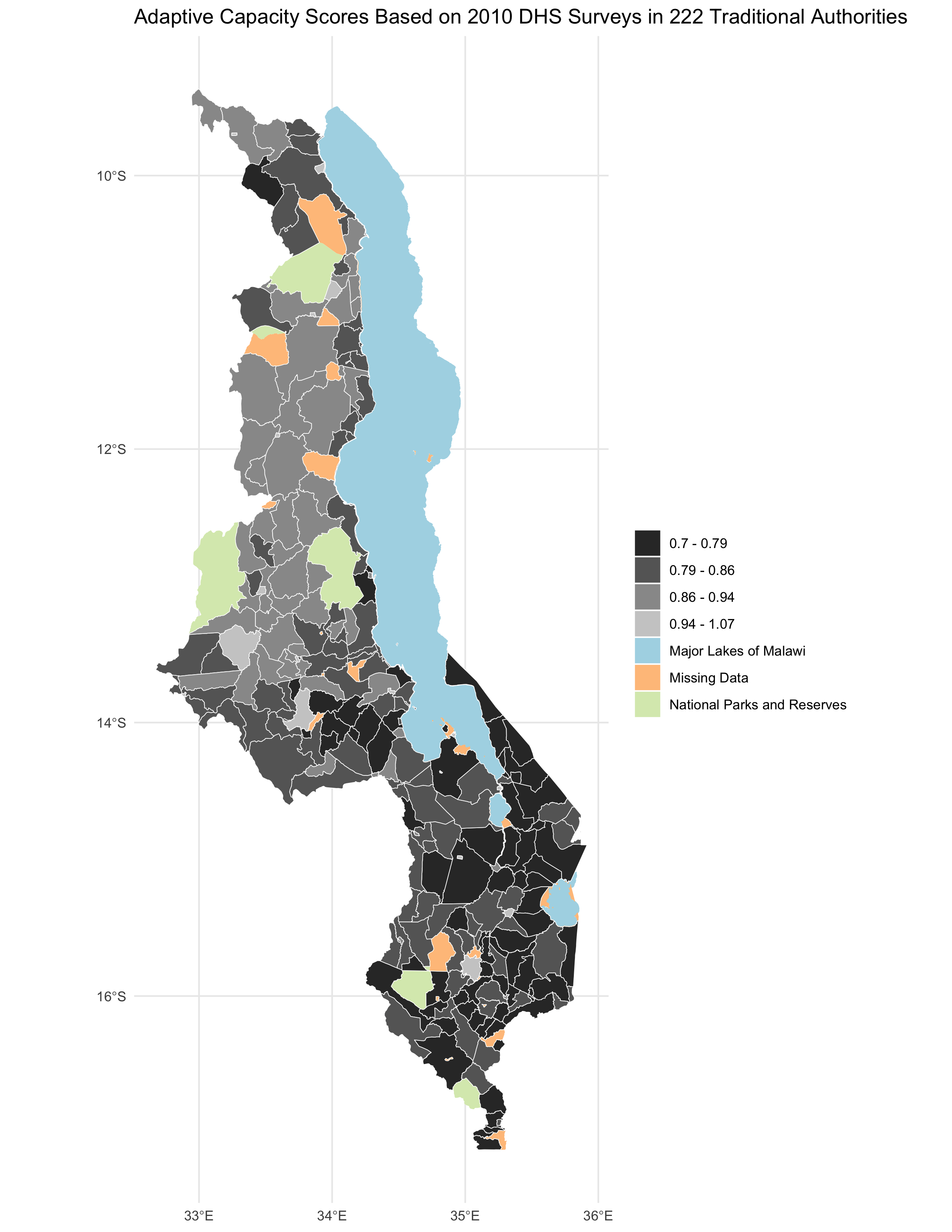
Figure 4: Adaptive Capacity
map of adaptive capacity by traditional authority in 2010, analagous to figure 4 of the original study
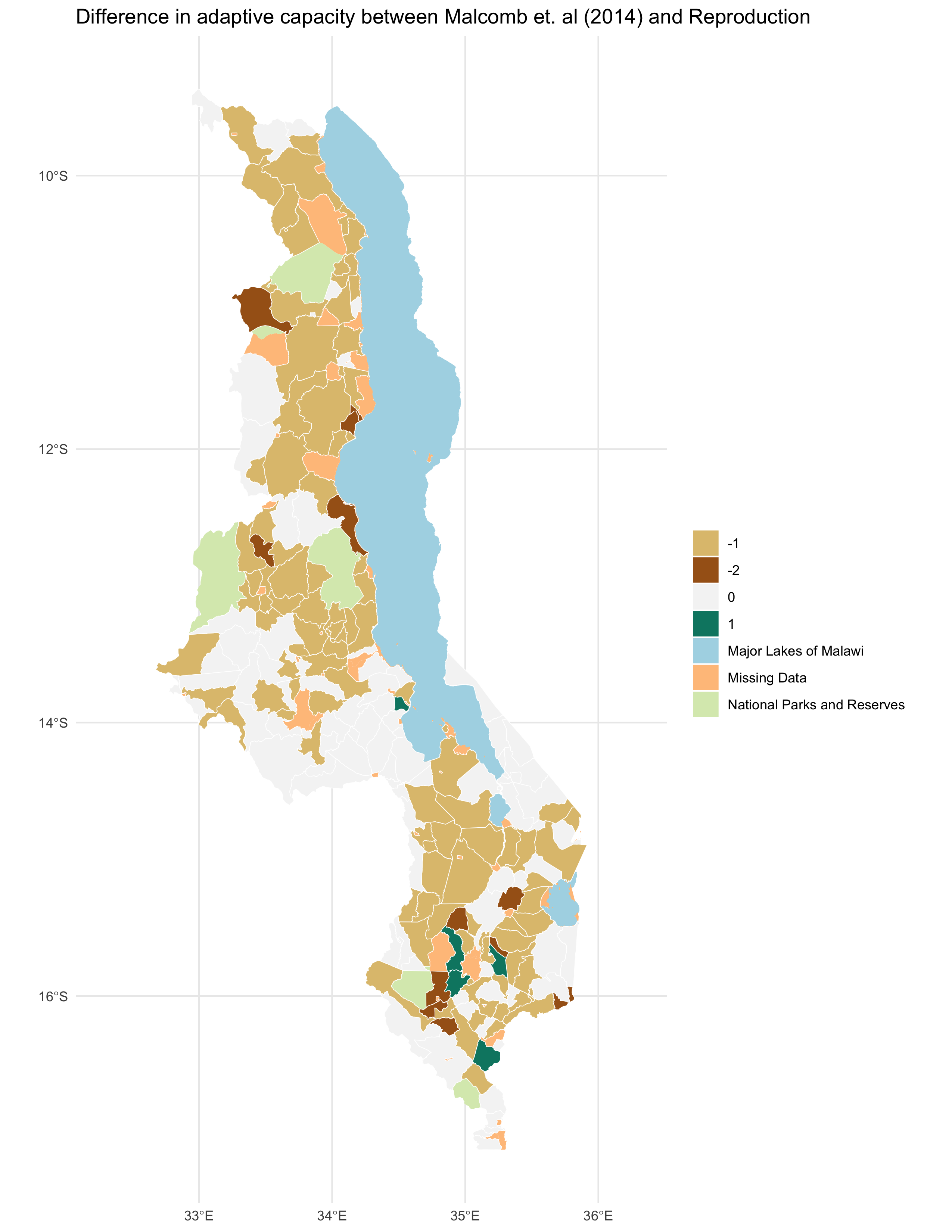
map of difference between your figure 4 and the original figure 4
Confusion Matrix
| 1 | 2 | 3 | 4 | |
|---|---|---|---|---|
| 1 | 35 | 5 | 0 | 0 |
| 2 | 27 | 26 | 0 | 0 |
| 3 | 5 | 44 | 19 | 0 |
| 4 | 0 | 7 | 28 | 4 |
Spearman’s Rho coefficients: Spearman’s Rho, Comparing figure 4: 0.7861
The calculation and visualization of the Adaptive Capacity was statistically by the reproduction, with a Spearman’s Rho value of 0.7861. Nevertheless, when looking at the confusion matrix, we see that the original study found a generally higher resilience/adaptive score than our reproduction (bottom-left skew in confusion matrix). This discrepancy is fairly low, with the vast majority of categories that were wrong as only one category off in either direction.
In the original study, the adaptive capacity scores range from 11 - 25, whereas those in the replication go from 0.7-1.07. In the given code written by Kufre Udoh and Joseph Holler, these values were multiplied by 20 to give a closer value to those in the original study. I removed this multiplication by 20 from our reproduction, as I believe that our code should attempt to independently reproduce the results, not match our approximate findings to the original through arbitrary data distortions. As seen below, I ignore this 20x distortion (using a # symbol) while still preparing the data for visualization breaks as created in the original study.
# join mean capacity to traditional authorities
ta = left_join(
  ta,
  select(ta_capacity_2010, ta_id, capacity_2010 = capacity_avg),
  by = c("ID_2" = "ta_id")
)

# making capacity score resemble malcomb et al's work
#ta = mutate(ta, capacity_2010 = capacity_2010 * 20)
# 256 features

# preparing breaks for mapping using natural jenks method
ta_brks = filter(ta, !is.na(capacity_2010)) %>% {classIntervals(.$capacity_2010, 4, style = "jenks")$brks}

#lapply: apply a function over a list or a vector
#make four classes of jenks for mapping/visualizing the data. Assign data to classes
ta_int = lapply(1:4, function(x) paste0(round(ta_brks[x],2)," - ", round(ta_brks[x +1],2))) %>% unlist()

ta = mutate(ta, capacity_2010_brks = case_when(
  capacity_2010 <= ta_brks[2] ~ ta_int[1],
  capacity_2010 <= ta_brks[3] ~ ta_int[2],
  capacity_2010 <= ta_brks[4] ~ ta_int[3],
  capacity_2010 >  ta_brks[4] ~ ta_int[4]
))
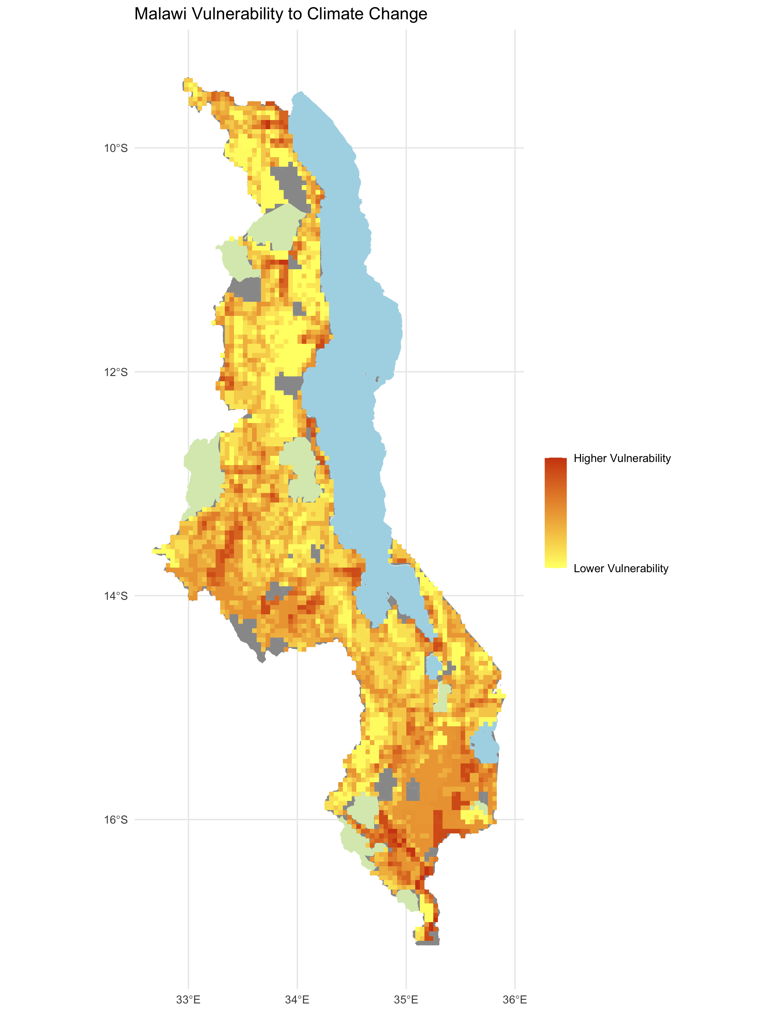
Figure 5: Vulnerability to Climate Change
map of vulnerability in Malawi, analogous to figure 5 of the original study
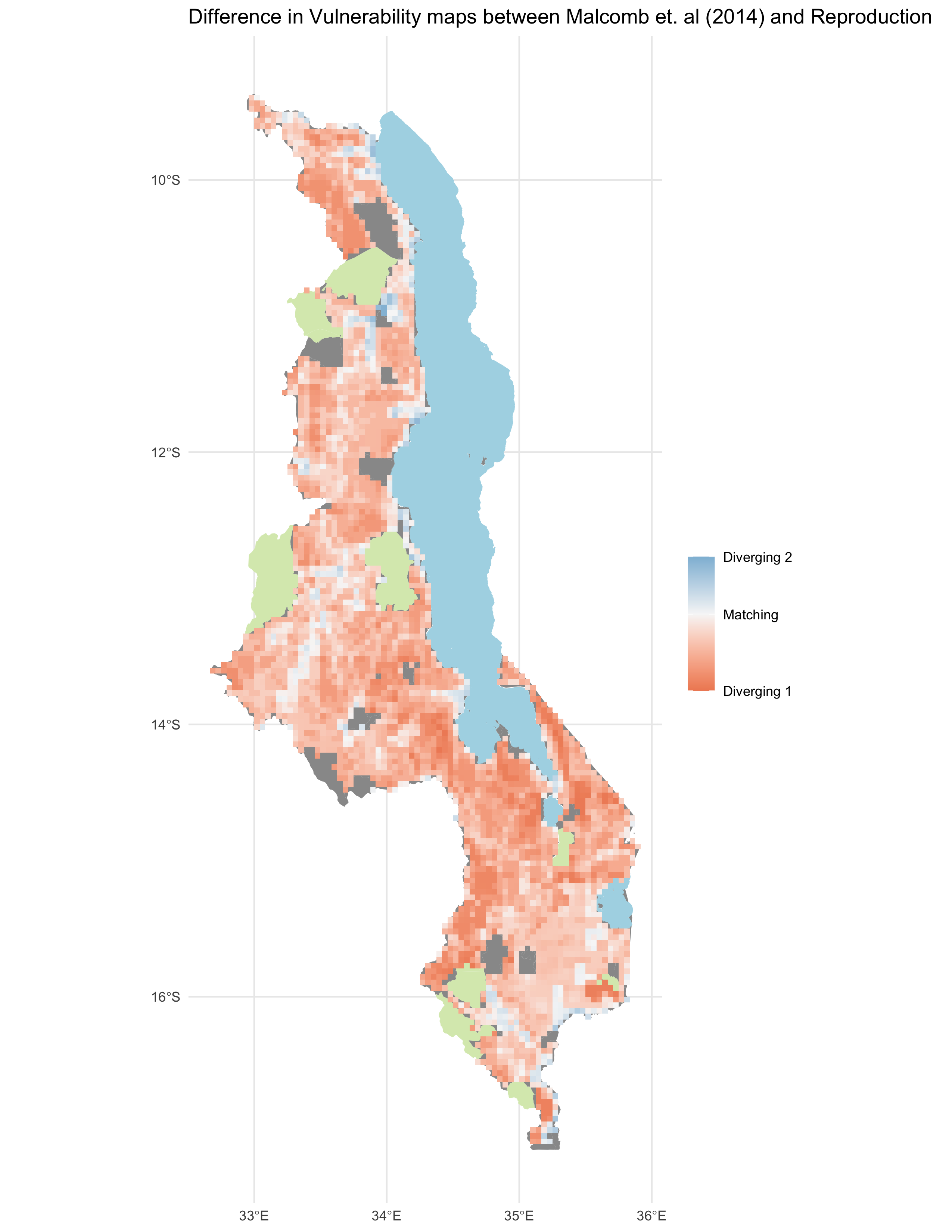
map of difference between your figure 5 and the original figure 5
Scatterplot of difference of results for Fig. 5
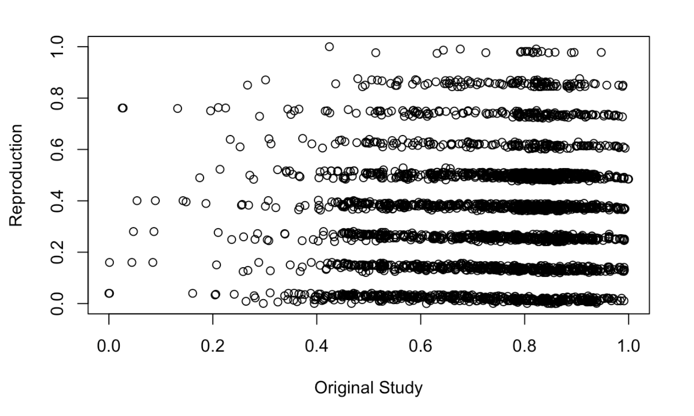
Spearman’s Rho coefficients: Spearman’s Rho, Comparing figure 5: 0.2244
Unlike the comparisons of the adaptive capacity maps, the vulnerability maps created in our reproduction align with those from Malcomb et al. (2014) to a much lesser degree. With a Spearman’s Rho of 0.224, there is little alignment between the two analyses. While the map of difference between my Figure 5 and the original Figure 5 shows some general alignment in vulnerability scores in southern and central Malawi, there is little alignment across other parts of the country.
I adjusted the function used to calculate vulnerability, especially the equation used in the final output. While the original study said that the vulnerability equation was Adaptive Capacity + Livelihood Sensitivity - Physical Exposure, the original equation provided in the reproduction code was final = (40 - geo) * 0.40 + drought * 0.20 + flood * 0.20, this does not account for the livelihood zones, nor the direct subtraction of physical exposure from the resilience scores. I attempted to adjust the resilience calculation to final = ((geo) * 0.6)) - (drought * 0.20 + flood * 0.20), but this yielded an even lower Spearman’s Rho coefficient, around 0.06. In the end, I struck a balance between aggregating in the livelihood zone scores and normalizing all the data to the same scale. The final code for calculating the vulnerability score can be seen below.
  # final output (adding component rasters)
  final = ((60-geo) * 0.6) + (drought * 0.2 + flood * 0.2)
}
Unplanned Deviations from the Protocol
Though we have listed our original workflow prior to analysis above, this was not the exact workflow we used in the final analysis. Our R-markdown code for Rstudio depicts the final workflow in code format, and is verbally written out below. Our original workflow plan was fairly similar to the plan we ended up using, albeit with far more specificity in the specific variables and calculations used. We were able to include the livelihood zone data after accessing the data and better understanding the shape of the data. As a group, we decided which variables would be used to create the livelihood zones (Table 2) based on references centered around page 21 in Malcomb et al. (2014). The original report is unclear in which variables were used to calculate the livelihood zone scores, along with if these data were from only the “poor” category or also included those in the “middle-class” and “rich” calculations of livelihood sensitivity. Aside from uncertainty in variables selected in the DHS and LHZ data, factors of normalization (as derived from Table 2 in Malcomb et al. (2014) (pg. 23)) used throughout our code replication do not yield the same results as the Malcomb report. As noted earlier, the adaptive capacity scores in our maps and those from Malcomb et al. (2014) do not align without an arbitrary multiplier of 20 prior to displaying in a map. Much of my interest in this report was focused on determining the how to align our results with those in the Malcomb report through normalization factors, but with no major breakthroughs. Additionally, Malcomb et al. (2014) claim to use quintiles for their categorization, but list these quintiles as ranging from 0-5 (representing six categories). This uncertainty is a area for future analysis, illustrating the importance of transparent code by researchers who are working to create replicable tools for assessing vulnerability.
Table 2 from Malcomb et al.(2014) – Calculating Household Resilience Score
Process Adaptive Capacity
- Bring in DHS Data [Households Level] (vector)
- Bring in TA (Traditional Authority boundaries) and LHZ (livelihood zones) data
- Get rid of unsuitable households (eliminate NULL and/or missing values)
- Join TA and LHZ ID data to the DHS clusters
- Pre-process the livestock data, Filter for NA livestock data, Update livestock data (summing different kinds)
- FIELD CALCULATOR: Normalize each indicator variable and rescale from 1-5 (real numbers) based on percent rank
- FIELD CALCULATOR / ADD FIELD: Apply weights to normalized indicator variables to get scores for each category (assets, access)
- SUMMARIZE/AGGREGATE: find the stats of the capacity of each TA (min, max, mean, sd)
- Join ta_capacity to TA based on ta_id, (Multiply by 20–meaningless??) I have a question about this (so do I) ln.216
- Prepare breaks for mapping –> Class intervals based on capacity_2010 field –> Take the values and round them to 2 decimal places –> Put data in 4 classes based on break values
- Save the adaptive capacity scores
Process Livelihood Sensitivity
- Load in LHZ csv into R
- Join LHZ sensitivity data into R code
- Create livelihood sensitivity score data based on breakdown provided in report (Table 2)
Process Physical Exposure
- Load in UNEP rasterSet CRS for drought
- Set CRS for flood
- Clean and reproject rasters
- Create a bounding box at extent of Malawi, Add geometry info and precision (st_as_sfc)
- RASTERIZE the adaptive capacity data with pixel data corresponding to capacity_2010 field
- RASTERIZE the livelihood sensitivity score with pixel data corresponding to capacity_2010 field
- SUM RASTERS: Combine adaptive capacity and livelihood sensitivity rasters
- For Drought: use bilinear to average continuous population exposure values
- For Flood: use nearest neighbor to preserve integer values
- RASTER CALCULATOR: a) Create a mask; b) Reclassify the flood layer (quintiles, currently binary); c) Reclassify the drought values (quantile [from 0 - 1 in intervals of 0.2 =5]); d) Add component rasters for final weighted score of drought + flood; e) Combine with adaptive capacity and livelihood zone data
- CLIP the traditional authorities with the LHZs to cut out the lake
- AGGREGATE: Create final vulnerability layer using environmental vulnerability score and ta_capacity
Discussion
Based on the research by Eric Tate (2013) around vulnerability modelling and uncertainty, we can better assess the framweorks used by Malcomb et al. (2014) to model vulnerability in Malawi. Malcomb et al. (2014) use a hierarchical model structure to index and combine variables for vulnerability mapping. This hierarchy was created through a deductive, normative, and practical approach, where researchers consulted with experts (who had often collected the existing data themselves), determined how community values are represented in existing variables, and constructed their analysis based on the data that was readily available. The analysis was conducted at the Traditional Authority and Livelihood Zone scale, and later rasterized to match the format of existing drought and and flood data in Malawi. Data was normalized to 0-5 quintiles and was weighted based on the normative judgements of research about what attributes contribute the most about vulnerability. Some variables, such as owning a phone or T.V., might signal societal trends and be used as proxies for wealth in adaptive capacity scores. Final outputs were constructed through aggregation to Traditional Authority boundaries and additive raster algebra. Uncertainty in the data and results was ignored in the final report, with the mean outputs being visualized and not investigating margins of error and statistical significance of findings. This uncertainty could have been assessed through a Monte Carlo simulation of different variables and weightings throughout the code, illuminating how much the choices of researchers affect final vulnerability outcomes.
Our attempt to reproduce this code was successful in creating vulnerability models for Malawi, but often did not match the original results by Malcomb et al. (2014). This failure is likely due to a lack of transparent data collection, lack of associated code for processing this data, and a lack of clarity towards how this data was used and aggregated in the analysis. There is lots of uncertainty in the original Malcomb et al. (2014) paper, with concerns about how data is aggregated, the scale to which it is aggregated, how the data is proprotionally normalized, and statistical distribution of vulnerability scores. For example, while Malcomb et al. (2014) provides a breakdown of proportionality, they do not quantify any of these values nor the scale at which they should be processed. This reproduction helps to tease out which variables impact the study by observing where decisions influence the output maps. In this light, I wonder:
- How much does each subjective decision I make in my work impact the result?
- How much is the study dependent on specific community conditions?
- Can conducting reproductions (using the same data and techniques to attempt same outputs) help with vulnerability model uncertainty?
To the first question, this reproduction could be improved by creating functions and for-loops to explore all reasonable scenarios where there is uncertainty or extensive opportunities for human bias. Some examples of where these functions would be useful are selecting which sources of income should be counted as assets and determining which scales of aggregation (TA vs. district) should be allowed. Using a “Monte Carlo” simulation that generates thousands of possibilities and combinations of variables and weightings in the data, we could determine more clearly how Malcomb et al. (2014) constructed their initial analysis. While it is inappropriate to “nudge” our results to align with the original results from Malcomb et al. (2014), a Monte Carlo simulation could expose these uncertainties and lack of transparency in uncertainty analyses (Tate 2013).
In response to if this study is dependent on specific community conditions, I am beginning to recognize the challenges with using index analyses to model livelihood patterns. In conversations with Professor Jessica L’Roe over the past two years, we have often gone back and forth on the validity of normalizing and indexing spatial data in analyses of access and vulnerability. After completing this reproduction, I am in greater agreement with Professor L’Roe on the challenges of using indices and the importance of running statistical tests to determine the accuracy of spatial models in relationship to lived experiences. In our work with the Basic Needs Survey (BNS) conducted by the Wildlife Conservation Society in 50+ villages in 10 landscapes across West, Central, and East Africa, we emphasized multi-variate statistical tests with existing data, as opposed to normalizing and aggregating our results. While the outputs may have been less visually appealing than the maps in this reproduction, Professor L’Roe’s emphasis on the robustness of data and mitigating uncertainty has helped apply our initial analysis of the Ituri landscape to the nine other landscapes in the study.
Conclusion
This analysis illuminates the difficulties of reproducing existing scientific work and the value of transparent code in conducting more robust reserach. While our map of Adaptive Capacity in the Traditional Authority boundaries comes fairly close to matching the results from Malcomb et al. (2014), our results do not align as well with the rasterized vulnerability map. The possible reasons for this inaccuracy and irreplicability are many, all based around a lack of transparency within the initial analysis towards data, aggregation, code, and processing capacities. These findings suggest a need for future reproductions of existing research that purport to provide replicable models of vulnerability and well-being across landscapes. For Malcomb et al. (2014) to truly have a replicable model for assessing vulnerability to climate change in landscapes outside Malawi, we first need to be able to reproduce this exact study in the original landscape. Only then will we have an additional tool for assessing vulnerability to climate change, and even then, we will need to factor in unique, local conditions to make these models beneficial in the lives of those who will be most harmed by these natural disasters.
References
Malcomb, D. W., E. A. Weaver, and A. R. Krakowka. 2014. Vulnerability modeling for sub-Saharan Africa: An operationalized approach in Malawi. Applied Geography 48:17–30. DOI:10.1016/j.apgeog.2014.01.004
Tate, E. 2013. Uncertainty Analysis for a Social Vulnerability Index. Annals of the Association of American Geographers 103 (3):526–543. doi:10.1080/00045608.2012.700616.
Background reserach informing this report (not directly cited in report)
Flanagan, B., E. Hallisey, J. D. Sharpe, C. E. Mertzlufft, and M. Grossman. 2020. On the Validity of Validation: A Commentary on Rufat, Tate, Emrich, and Antolini’s “How Valid Are Social Vulnerability Models?” Annals of the American Association of Geographers 0 (0):1–6. DOI:10.1080/24694452.2020.1857220.
Rufat, S., E. Tate, C. T. Emrich, and F. Antolini. 2019. How Valid Are Social Vulnerability Models? Annals of the American Association of Geographers 109 (4):1131–1153. DOI:10.1080/24694452.2018.1535887.
Rufat, S., E. Tate, C. T. Emrich, and F. Antolini. 2020. Answer to the CDC: Validation Must Precede Promotion. Annals of the American Association of Geographers 0 (0):1–3. DOI: 10.1080/24694452.2020.1857221.
Sergio Rey - AAG Annual Meeting on Big Code
Report Template References & License
This template was developed by Peter Kedron and Joseph Holler with funding support from HEGS-2049837. This template is an adaptation of the ReScience Article Template Developed by N.P Rougier, released under a GPL version 3 license and available here: https://github.com/ReScience/template. Copyright © Nicolas Rougier and coauthors. It also draws inspiration from the pre-registration protocol of the Open Science Framework and the replication studies of Camerer et al. (2016, 2018). See https://osf.io/pfdyw/ and https://osf.io/bzm54/
Camerer, C. F., A. Dreber, E. Forsell, T.-H. Ho, J. Huber, M. Johannesson, M. Kirchler, J. Almenberg, A. Altmejd, T. Chan, E. Heikensten, F. Holzmeister, T. Imai, S. Isaksson, G. Nave, T. Pfeiffer, M. Razen, and H. Wu. 2016. Evaluating replicability of laboratory experiments in economics. Science 351 (6280):1433–1436. https://www.sciencemag.org/lookup/doi/10.1126/science.aaf0918.
Camerer, C. F., A. Dreber, F. Holzmeister, T.-H. Ho, J. Huber, M. Johannesson, M. Kirchler, G. Nave, B. A. Nosek, T. Pfeiffer, A. Altmejd, N. Buttrick, T. Chan, Y. Chen, E. Forsell, A. Gampa, E. Heikensten, L. Hummer, T. Imai, S. Isaksson, D. Manfredi, J. Rose, E.-J. Wagenmakers, and H. Wu. 2018. Evaluating the replicability of social science experiments in Nature and Science between 2010 and 2015. Nature Human Behaviour 2 (9):637–644. http://www.nature.com/articles/s41562-018-0399-z.