Jacob Freedman's Portfolio
webpage portfolio for open source GIS work
Project maintained by jafreedman12 Hosted on GitHub Pages — Theme by mattgraham
RE- Replication of Rosgen Stream Classification
Replication of
A classification of natural rivers
Original study by Rosgen, D. L. in CATENA 22 (3):169–199. https://linkinghub.elsevier.com/retrieve/pii/0341816294900019.
and Replication by: Kasprak, A., N. Hough-Snee, T. Beechie, N. Bouwes, G. Brierley, R. Camp, K. Fryirs, H. Imaki, M. Jensen, G. O’Brien, D. Rosgen, and J. Wheaton. 2016. The Blurred Line between Form and Process: A Comparison of Stream Channel Classification Frameworks ed. J. A. Jones. PLOS ONE 11 (3):e0150293. https://dx.plos.org/10.1371/journal.pone.0150293.
Replication Authors: Jacob Freedman, Zach Hilgendorf, Joseph Holler, and Peter Kedron.
Replication Materials Available at: Re-Rosgen
Created: 19 March 2021
Revised: 24 March 2021
Land Acknowledgement: This analysis takes place on the traditional lands of the Cayuse, Umatilla and Walla Walla and the Confederated Tribes of Warm Springs.
Abstract
In this study, we are replicating Rosgen’s (1994) seminal classification of river systems, an effort that was originally undertaken to make the understanding of rivers transferable across disciplines. By looking at the surrounding landscape and the composition of the river, Rosgen (1994) hypothesized that a river classification system could be created and replicated for use in multiple disciplines. While previous studies attempted to classify streams based on age (Davis 1899), slope (Schumm 1963), bedload (Schumm 1977), valley pattern (Thornbury 1969), and pattern of movement (Brice and Blodgett 1978), among with many others, each of these was not effective for classifying streams across a variety of landscapes. By combining elements from all of these previous classifications, Rosgen focused on sinuosity, entrenchment, and widths of flood-prone areas to construct a multi-level classification system that emphasized the hierarchies of “states” of a river. Building on this research, Kasprak et al. (2016) set out to examine the replicability and accuracy of the Rosgen Classification System (along with other classification systems), using spatial analysis tools at a watershed scale. Looking at the Middle Fork of the John Day River watershed, Kasprak et al. (2016) used DEM data and field-collected river data
In this analysis, we are working to replicate the Rosgen classification system as replicated by Kasprak et al. (2016), all while using open-source GIS resources. By testing this replicability, we hope to better understand if these kind of river analyses can be achieved entirely with open-source GIS tools.
Original Study Information
While Rosgen (1994) provides a framework for the Rosgen Classification System at various levels (relevant here are Level I: general landscape form, and Level II: more specific, field-based measurements), the research by Kasprak et al. (2016) provides an opportunity for us to replicate an existing automation of a framework. One of the major challenges with river classification is the variability between classification systems and the need for data gathered in the field. While both our analysis and that by Kasprak et al. (2016) use information from the field about stream bed composition, the capacity to do a large portion of these analyses using aerial imagery and GIS reflects immense possibilities in the easier replication and comparison of river classification systems.
For the purposes of this report, I will focus on the use of the Rosgen Classification System (RCS) by Kasprak et al. (2016), although they compared this analysis with the River Styles Framework, the Columbia Basin Natural Channel Classification, and a Statistical Classification. Kasprak et al. (2016) set out to classify rivers at the watershed scale, using the Middle Fork of the John Day River Watershed (MFJD) as a test location. With an immense amount of field data collected for this site because of salmon monitoring, it was possible to complete the RCS and the other classifications without needing to collect river samples on their own. Using 33 points of analysis from the CHaMP (Columbia Habitat Monitoring Program) dataset, Kasprak et al. (2016) used 10m and 0.1m DEMs 1m aerial imagery to determine the Level I classifications at each CHaMP point. Classifications of width-depth ration, sinuosity, entrenchment, and gradient were calculated from O.1m DEMs and the River Bathymetry Toolkit.
The data from this original analysis can be found in our publicly-available “Re-Rosgen”repository. CHaMP shapefiles and DEM data for the John Day Watershed can be found at the corresponding links.
Sampling Plan and Data Description
Figure 1: Point of analysis (Location 13) in the CHaMP dataset in the MFJD watershed
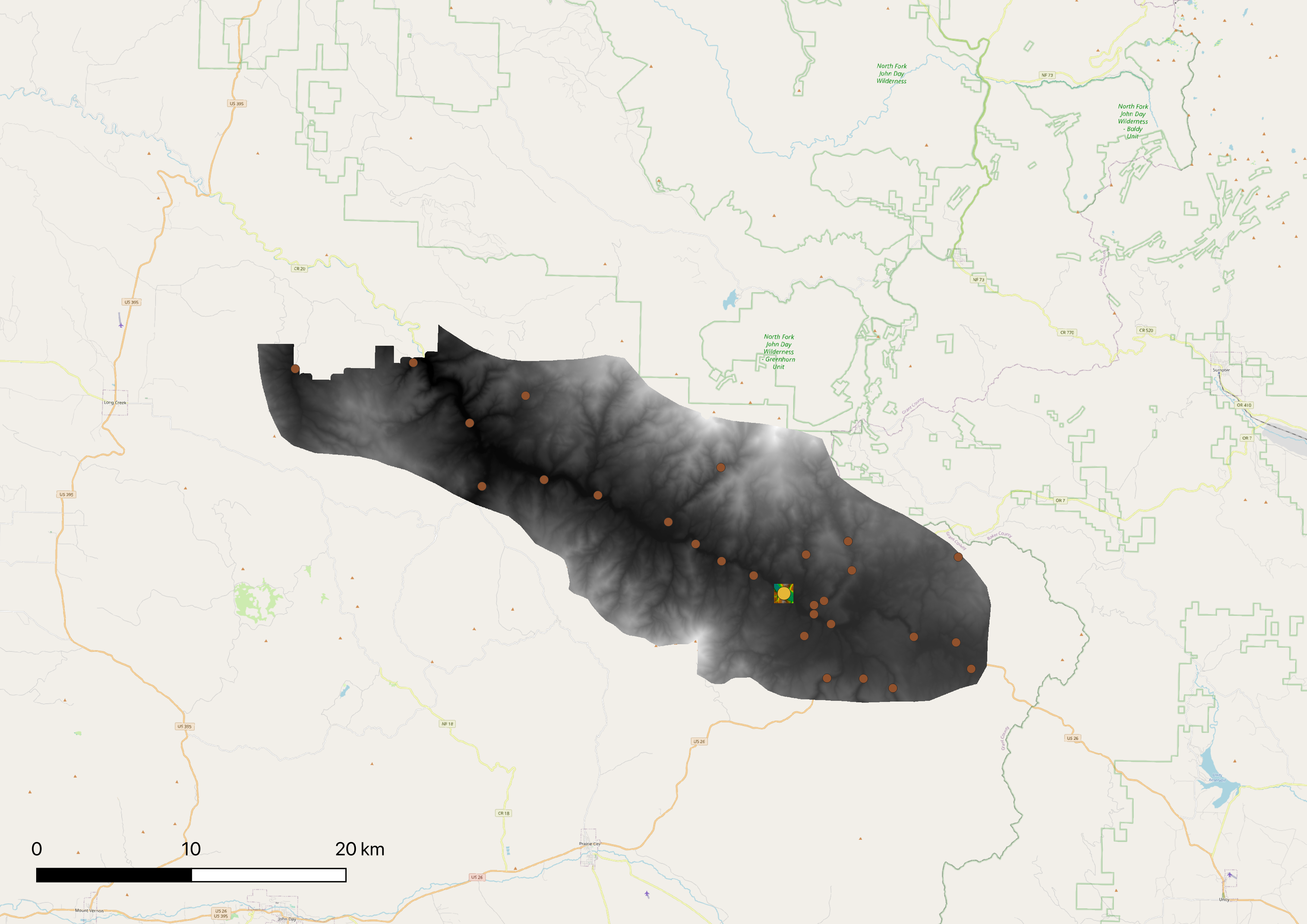
The data collected for this analysis was performed primarily using the CHaMP dataset of river depth and quality throughout the John Day watershed, a dataset created in the monitoring of salmon populations. 33 sites were randomly selected by Kasprak et al. (2016), and in our class of 18 students, we were each randomly assigned a study site for this analysis. I was assigned Location 13 (Figure 1). 10m DEM data is publicly available across the United States through the USGS 3DEP program. We received this DEM as pre-processed LiDAR for the extent of the John Day watershed at a 1m pixel resolution, though the authors state they used 10m and 0.1m pixels for their DEM analyses. This 0.1m DEM was likely derived from LiDAR point cloud data.
Kasprak et al. (2016) performed this analysis on 33 sites in the MFJD watershed, using the average of 100+ , 1m-spaced cross-sections at each site to help with the classification of each river in the RGS framework. They used a generalized random tessellation stratified sampling method to select the 33 CHaMP sites (sampled in 2012 and 2013) that were eventually used in this analysis. While the authors do not make clear the origins for their DEM data, it is fairly easy to find high-quality DEM and aerial imagery in the United States through the USGS 3DEP program. The CHaMP data for 2012 and 2013 was gathered in collaboration with the Columbia Habitat Monitoring Project, and the authors make clear that this research is a project for the CHaMP Monitoring Project.
Variables – Describe the variables used in the original study to address the research questions and hypotheses that are the focus of the replication.
The river classifications in this study were determined from stream characteristics that come from the surrounding landscape relief, landform, and valley morphology. By calculating the slope (change in elevation/change in distance), sinuosity (channel length/valley length), width:depth ratio (bankfull width/bankfull depth), and entrenchment ratio (width of flood-prone area/width of bankfull river, where the width of the flood-prone area is determined at twice the maximum bankfull depth) of the river, the authors of Kasprak et al. (2016) were able to classify each of the rivers at the 33 sampled points into the Rosgen System of River Classification. Bankfull is defined as the initial point of river flooding – a significant detail for river classification, especially concerning the determination of floodplain extent.
Table 01. Ratios used in Rosgen Classification System
| Ratio type | Calculation |
|---|---|
| Entrenchment Ratio | width of flood-prone area/width of bankfull river, where the width of the flood-prone area is determined at twice the maximum bankfull depth |
| Width / Depth Ratio | bankfull width/bankfull depth |
| Sinuosity | channel length/valley length |
Analytical Specification
With no guiding hypotheses in this study and a greater emphasis on testing research design, there is little to report in analytical specifications. Kasprak et al. (2016) place a larger emphasis on automating and comparing multiple river classification schemes and, for our purposes, understanding how this classification will work for the Rosgen Classification System.
Materials and Procedure
This report is to assess if the watershed-scale classifications by Kasprak et al. (2016) can be entirely replicated with open-source GIS and statistical software. Using GRASS, QGIS 3.16 LTR, RStudio, and Github as a data and procedure repository. It is presumed that the original replication study occurred using ArcGIS and other proprietary softwares, though this is not made clear in the paper. Both our study and Kasprak et al. (2016) use the CHaMP points for specific site classification, with Kasprak using points from 2012-2013 and ours ranging from 2011-2017. At my site (location 13) there were four sampled points from 2013-2015, and my random selection led to using one of the 2013 points for this study.
Protocol
Both Kasprak et al. (2016) and our replication follow the Rosgen Classification System template for classifying the river to Level I and Level II specifications. While Kasprak used the River Bathymetry Toolkit (RBT), a set of river analysis tools designed to function with ArcGIS desktop, we did many of these same steps with manual digitization and terrain analysis in GRASS.
For our replication, we began with a workspace in GRASS for doing our terrain processing. Working in the projection NAD 1983 UTM Zone 11 North, we loaded in the 1m LiDAR-derived DEM of the watershed and all relevant points from the CHaMP dataset. To create our study region, we built a buffer of 20 channel widths around our selected point of interest (e.g. location 13 (Fig. 1)), created a square analysis region around the buffer, and clipped the LiDAR-derived DEM to that analysis region. A hillshade and slope were applied to the elevation data, to be used in subsequent classifications. To determine the length of the river and valley, the river banks and valley banks were each manually digitized three separate times at a scale of 1:1500. Since my valley borders were outside the extent of the buffer, I expanded my digitization scale to 1:2500 for the valley digitization. Each of these three classifications was done alternating over the preprocessed hillshade and slope classifications, so as to avoid biases from re-replicating our first digitization attempts over and over again. Following the digitization, a composite centerline for the valley and river were constructed from the centerlines of all three digitization attempts (Fig. 4; Fig. 5). The river centerline was exported to Rstudio as a text files of points containing elevation data for each location at 100m intervals along the river. A transect of the valley was constructed at the location of CHaMP location 13, and was similarly exported to RStudio for post-processing and analysis. With all these calculations supplemented with site-specific details (bankfull depth, particle size, etc.), the Rosgen Classification could be replicated.
For replication in another raster-processing program, complete the following steps:
- Create hillshade and slope
- Digitize river banks and valley edges over multiple (3) digitizations
- Find the average (middle line) of each of these digitizations
- Construct a longitudinal profile of the river
- Construct a cross-sectional profile of the river at the location of analysis/interest.
The main differences from the original study (Kasprak et al. 2016) are that this replication uses open-source software and does not have access to the RBT toolkit. The RBT toolkit in ArcGIS allows uses to automatically calculate the slope, bankfull width and depth, sinuosity, and all other features (excluding particle size) found in Table 2. Kasprak ran their RCS classifications on 33 points, whereas our class of 18 students only managed to classify 18 locations. Our DEM data is at a grainer resolution (1m as compared to 0.1m), though both of these resolutions are incredible and fairly accurate for the method of classification. Nevertheless, there are some hash-line artifacts in the elevation data, perhaps from automated processing within the USGS.
To determine if our replication was successful, we will compare our Rosgen river classifications to those provided in the CHaMP dataset to determine the similarity of our results.
Replication Results
This replication was undertaken at one location in the CHaMP dataset. For the Level I classification, bankfull width, depth, and average particle size were derived from the CHaMP dataset, stream and valley length were calculated within the same buffer region in GRASS, valley width was calculated in RStudio, and valley depth was derived from bankfull depth from CHaMP data (Table 2). Entrenchment, width:depth, and sinuosity were derived from these calculations, allowing us to determine that the Level I classification was C, a river with a low-sloping, relatively developed floodplain (Table 3; EPA 2005). By deriving the river slope from the change in height divided by the change in length throughout the sample buffer region, slope could be calculated for the Level II classification (Table 4). Combined with a chart from our protocol handbook, we determined the channel material class based on the average particle size from Table 2, helping us classify this river as a C4 river (Figure 8; Table 4).
This result does not match the classification for this point from the classification done by Kasprak et al. (2016), which found this specific point in 2013 to be a B3c river (VisitID 1903 at loc_id 13). Nevertheless, the other three classifications for this point in the river, from 2013, 2014, and 2015, found that the RCS was either C3b (2013) or C4b (2014 & 2015). The presence C4b aligns with the findings from Kasprak et al. (2016), where 24% of all findings were in this category. Similarly, 50% of findings were in the B stream classification, which reflects Kasprak’s findings for this site in 2013. Despite all of these differences at different years, Table 5 in Kasprak et al. (2016) states that this site (defined as CBW05583-449266) is a C4b river in the Rosgen Classification System.
Figures and Tables
Figure 2: Slope at location 13
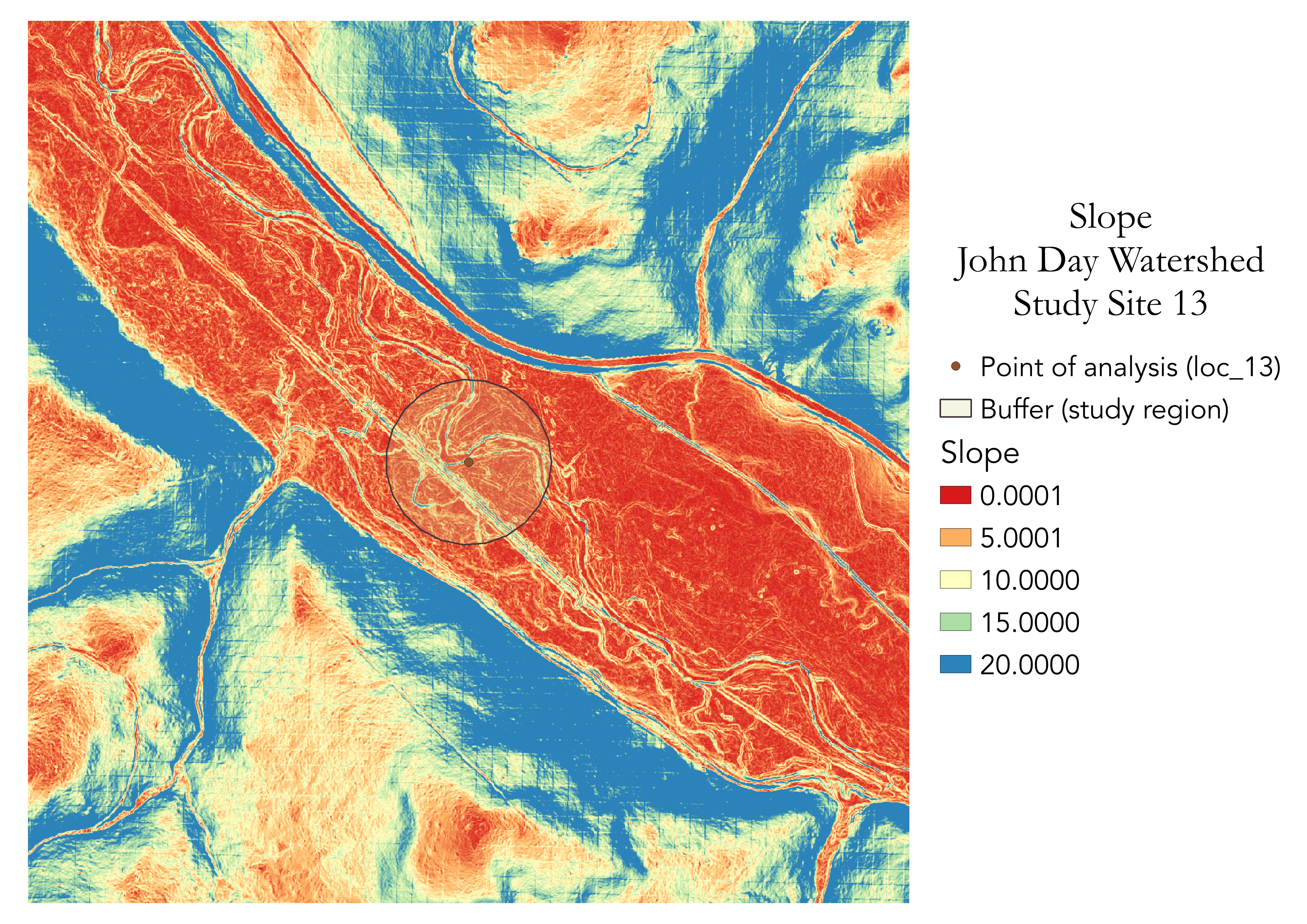
Figure 3: Shaded elevation at location 13
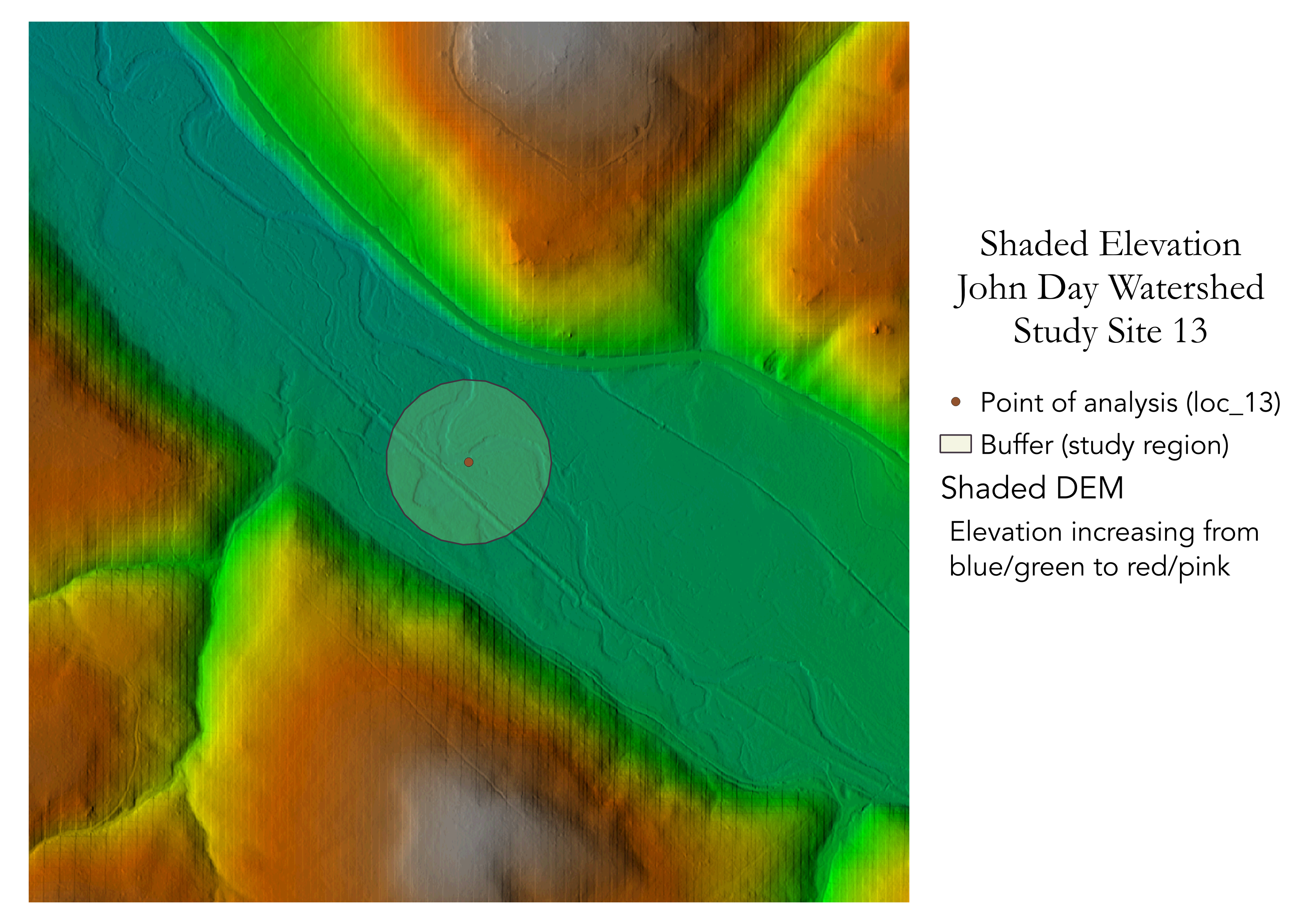
Figure 4: Composite stream centerline
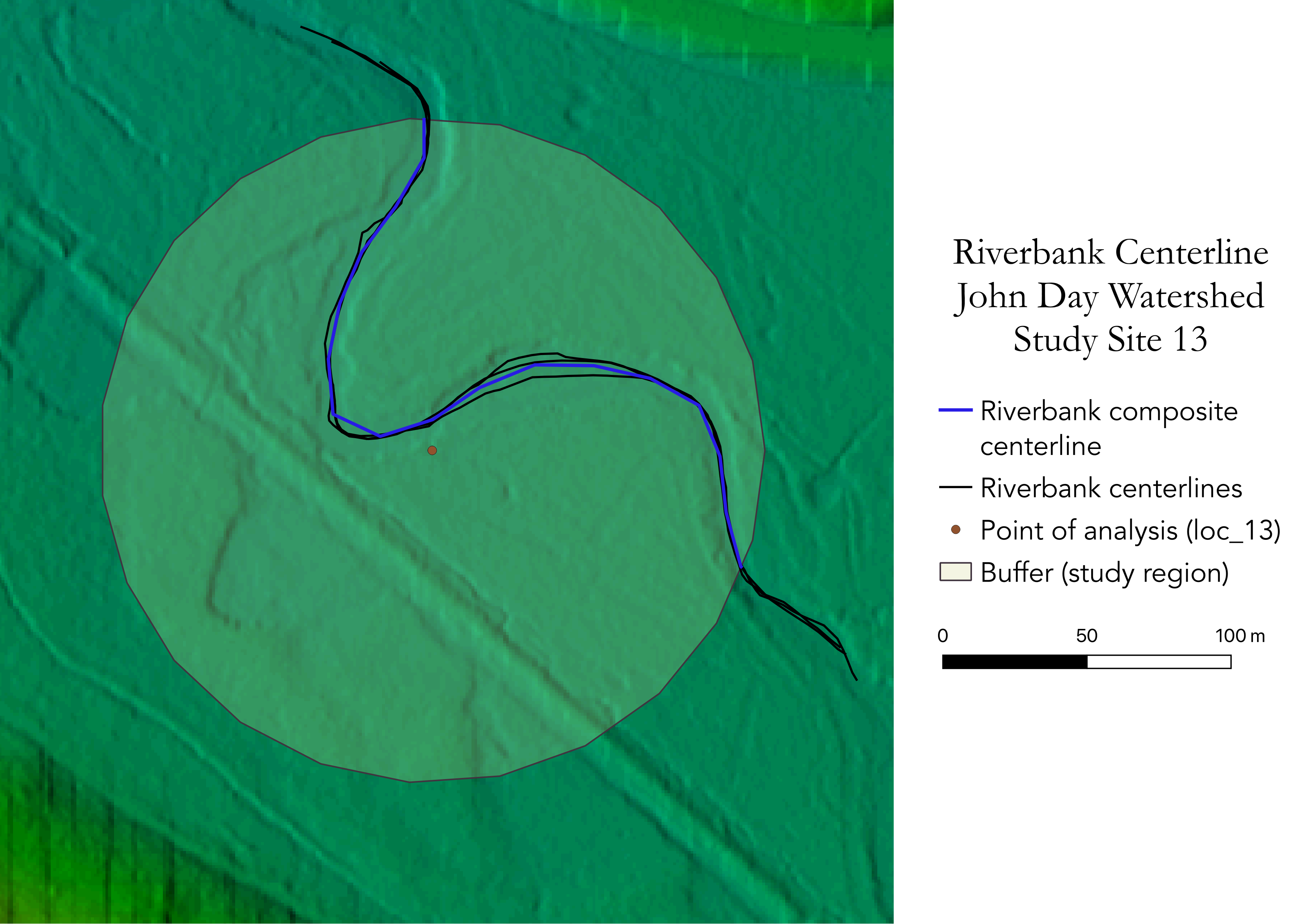
Figure 5: Composite valley centerline
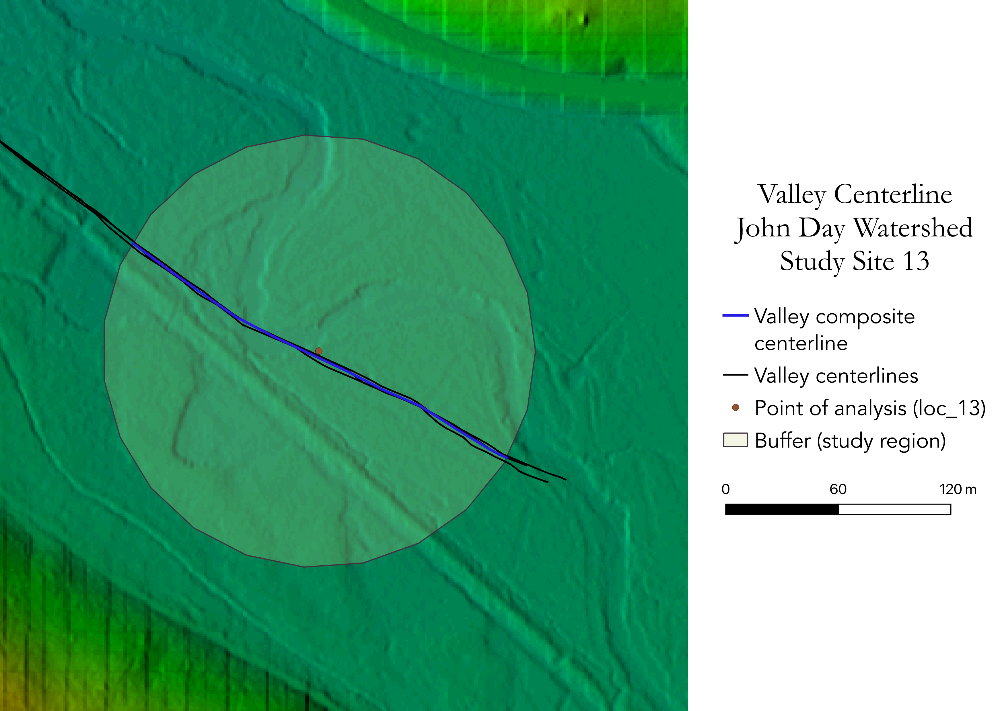
Figure 6: Longitudinal profile of river
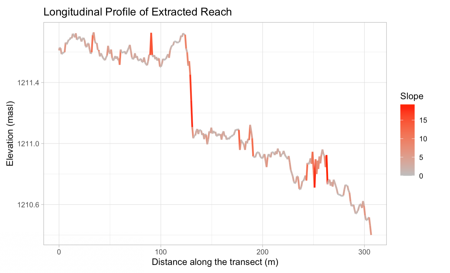
Figure 7: Cross-sectional river profile
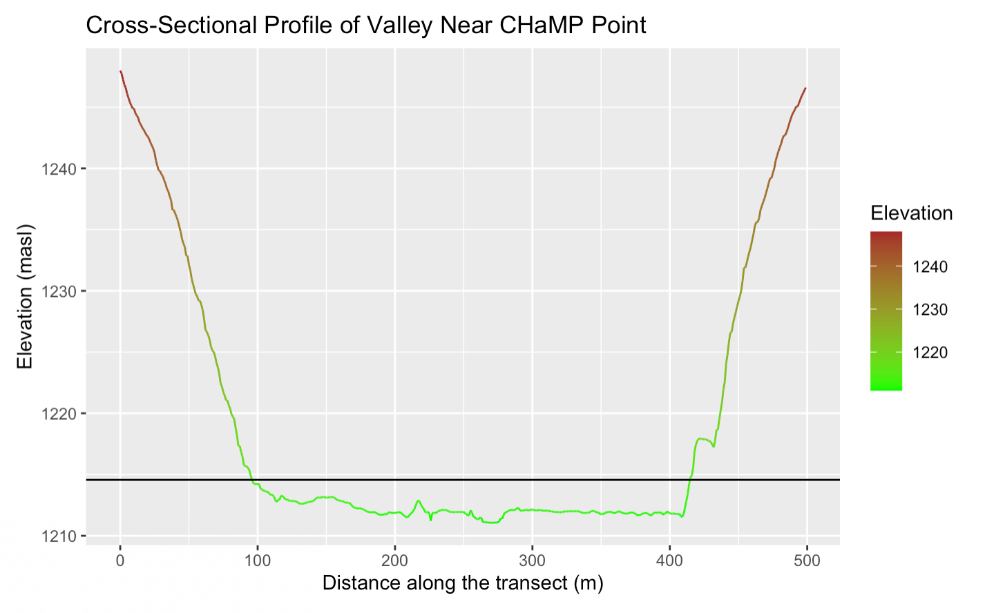
Figure 8: Annotated flow chart of Rosgen Classification System
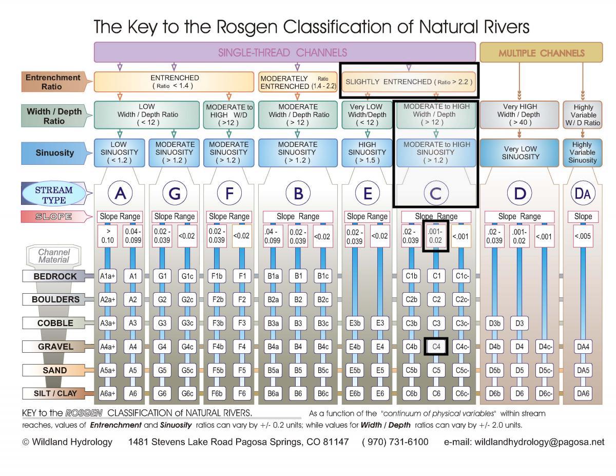
Table 2. Site Measurements
| Variable | Value | Source |
|---|---|---|
| Bankfull Width (m) | 8.0755 | CHaMP_Data_MFJD |
| Bankfull Depth Average (m) | 0.4031 | DpthBf_Avg in CHaMP_Data_MFJD |
| Bankfull Depth Maximum (m) | 1.7449 | DpthBf_Max in CHaMP_Data_MFJD |
| Valley Width (m) | 325 | Figure 7: Cross-sectional river profile |
| Valley Depth (m) | 3.4998 | Bankfull Depth Maximum x2 |
| Stream/River Length (m) | 306.66 | calculation in buffer GRASS |
| Valley Length (m) | 230.17 | calculation in buffer region in GRASS |
| Median Channel Material Particle Diameter (mm) | 70 | SubD50 variable in CHaMP_Data_MFJD |
Table 3. Rosgen Level I Classification
| Criteria | Value | equation |
|---|---|---|
| Entrenchment Ratio | 325/8.0755= 40.23497 | |
| Width / Depth Ratio | 8.0755/0.4031=20.03349 | bankfull width/bankfull average depth |
| Sinuosity | 306.66/230.17=1.33232 | channel length/valley length |
| Level I Stream Type | C |
Table 4. Rosgen Level II Classification | Criteria | Value | | — | — | | Slope | 0.0074 (0.74%) | | Channel Material | Gravel | | Level II Stream Type | C4 |
Unplanned Deviations from the Protocol
The primary deviation from the protocol was needing to expand the scale of digitization for the valley, as the valley lines were beyond the scope of the buffer. While we were provided a later tool to not clip the valley boundaries to the extent of the buffer (if the valley length did not bisect the buffer), my lenght was generally near the center of the buffer and worked for calculating the sinuosity of the river (Table 3).
Discussion
All of my results for the Level I and Level II classifications were internally consistent, meaning that that they fit into the framework created by Rosgen (1994) (Fig. 8). It remains unclear if this assessment is an accurate replication of the findings by Kasprak et al. (2016). On one hand, the exact classification (B3c) for this point does not align with our classification of C4, yet the overall classification for all samples at this location (C4b) is far closer to our findings. It unclear which of the points from 2013 Kasprak used, especially since neither yields a C4b classification on their own. It is very possible that Kasprak used a different sample from 2012 or 2013 that classified this river as a C4b, but the results from the paper and the corresponding data in the CHaMP dataset fail to further illuminate on the subject.
There are certainly uncertainties and errors in the calculation of these variables, namely channel length, valley length, and slope. Since each of these variables was calculated in a contained buffer region, it is possible that the length and extent for valley/river length and height are different than in the Kasprak analyses. This could be especially pertinent towards why we classified our river as C4 and not C4b (Figure 8), as the slope of the river is directly related to sample region size. The manual digitization of river banks and valleys requires the researcher to have a working knowledge of stream form and digitization practices, and inherently incorporates numerous arbitrary decisions into the digitization, such as selecting a scale for digitization. This zooming in forces us to focus only on the study site and ignore the broader context of the river geomorphology and trends in floodplains across the landscape. By only comparing our analysis to the Rosgen Classification, our analysis is less robust than the comparative study undertaken by Kasprak et al. (2016) and only emphasizes certain physical properties of the landscape.
There are different methods of finding elevation data, from field measurements to derivations from DEM data of different resolution (10m vs. 1m vs. 0.1m pixels). These variances in resolution lead to different calculations of slope, an important variable in creating the Level II classification of the river. Because of our controlled study area of a circle with a radius of approximately 10 river widths, slope was manually calculated for only a small subsection of the river (Fig. 7).
It would be challenging to do this classification entirely in GIS and without any field data. We used the CHaMP dataset to determine the mean particle size and the bankfull width/depth. The bankfull river width measurements could theoretically be completed with GIS, though the depth would be more challenging due to reflectance on the water.
This overall uncertainty stems from the limited region of analysis and the scale at which this analysis is undertaken. Without physically visiting the site and incorporating perspectives of the surrounding landscape, any GIS analysis will inherently exclude certain regions in order to classify the specific region of investigation. This lack of external context can be ameliorated through replicating this analysis of a single point at different geographic scales, calculating the slope, river/valley length, and sinuosity at more zoomed-out scales. While this will not provide the same context as physically observing the landscape and validating findings through ground-truthing, creating samples with different underlying scales of data can help reduce uncertainty. Only with full opportunity to visit each site with a diverse team of scientists tangentially related to stream geomorphology could these uncertainties be minimized, and even then, biases of researchers and prior experiences in the field could create new uncertainties in our classifications.
Conclusion
The potential to replicate the Rosgen River Classification with open-source GIS tools is promising. While our classification for our randomly-selected sample point at our site did not yield the exact classification found by Kasprak et al. (2016), it matches more closely with the overall results of the paper that possibly summarized results from multiple different samples at the same (loc_13) site. These findings suggest a need for future investigations of how the classification of the same river at multiple time intervals can shift, and if these shifts are indicative of changes in river geomorphology or are more related to sampling difference. Similarly, this analysis would benefit from a larger spatial and temporal perspective that explores how the river is changing across a larger landscape. By completing this same analysis in multiple locations over a longer time span, GIS offers a promising solution for automating and tracking these changes over time in service of assessing patterns of river evolution.
References
- Hilgendorf, Z. & Holler, J. 2021. Primer for Rosgen Stream Classification course module. Arizona State University & Middlebury College.
- Kasprak, A., N. Hough-Snee, T. Beechie, N. Bouwes, G. Brierley, R. Camp, K. Fryirs, H. Imaki, M. Jensen, G. O’Brien, D. Rosgen, and J. Wheaton. 2016. The blurred line between form and process: A comparison of stream channel classification frameworks ed. J. A. Jones. PLOS ONE 11 (3):e0150293. https://dx.plos.org/10.1371/journal.pone.0150293.
- Rosgen, D. L. 1994. A classification of natural rivers. CATENA 22 (3):169–199. https://linkinghub.elsevier.com/retrieve/pii/0341816294900019.
Thank you to the entire GEOG0323 - Open Source GIS for their collaborative spirit and willingness to help troubleshoot questions throughout the assignment. Their support is what helps this work continue.
Report Template References & License
This template was developed by Peter Kedron and Joseph Holler with funding support from HEGS-2049837. This template is an adaptation of the ReScience Article Template Developed by N.P Rougier, released under a GPL version 3 license and available here: https://github.com/ReScience/template. Copyright © Nicolas Rougier and coauthors. It also draws inspiration from the pre-registration protocol of the Open Science Framework and the replication studies of Camerer et al. (2016, 2018). See https://osf.io/pfdyw/ and https://osf.io/bzm54/
Camerer, C. F., A. Dreber, E. Forsell, T.-H. Ho, J. Huber, M. Johannesson, M. Kirchler, J. Almenberg, A. Altmejd, T. Chan, E. Heikensten, F. Holzmeister, T. Imai, S. Isaksson, G. Nave, T. Pfeiffer, M. Razen, and H. Wu. 2016. Evaluating replicability of laboratory experiments in economics. Science 351 (6280):1433–1436. https://www.sciencemag.org/lookup/doi/10.1126/science.aaf0918.
Camerer, C. F., A. Dreber, F. Holzmeister, T.-H. Ho, J. Huber, M. Johannesson, M. Kirchler, G. Nave, B. A. Nosek, T. Pfeiffer, A. Altmejd, N. Buttrick, T. Chan, Y. Chen, E. Forsell, A. Gampa, E. Heikensten, L. Hummer, T. Imai, S. Isaksson, D. Manfredi, J. Rose, E.-J. Wagenmakers, and H. Wu. 2018. Evaluating the replicability of social science experiments in Nature and Science between 2010 and 2015. Nature Human Behaviour 2 (9):637–644. http://www.nature.com/articles/s41562-018-0399-z.